How this radar measures range, speed and direction
These notes follow the radar signal in the order it is actually processed — from the transmitted chirp and its reflected echo, through the Range and Doppler FFTs, to angle estimation, CFAR detection, tracking, and finally the ACC controller that acts on it.
Start by watching the vehicle and the radar plots together
Gazebo provides the simulated road, vehicles and reflections. ROS 2 carries the radar measurements and vehicle data between the processing, tracking and control nodes. The plots show the beat I/Q signal, Range FFT, Doppler FFT, Range–Doppler map and angle estimate, all produced from the same frame.
What to look for
- Range FFT — the peak position estimates target distance.
- Doppler FFT — the peak bin measures range rate across chirps.
- 3-D view — each point combines range, velocity and azimuth into one detection.
v_r ≈ v_lead − v_ego · positive means opening, negative means closing, zero means a constant gap. The selected Doppler value is relative radial velocity, not the lead vehicle's absolute speed.
Turn the echo into a slow signal the ADC can record
A 77 GHz wave is far too fast to digitise directly. The mixer removes the common fast motion and leaves only the small difference between the transmitted chirp and its delayed echo.
The echo is late, not different
Think of the radar sounding a note that steadily rises. The reflected copy returns after a delay τ. At any instant the transmitter has already climbed to a higher frequency while the echo is still repeating an earlier, lower one. That vertical gap is the beat frequency f_b.
Same slope. The echo is simply late.
The mixer exposes the difference
A mixer multiplies the transmitted reference by the received wave. The product contains one very fast sum term and one slow difference term; a low-pass filter removes the fast part. What remains is the beat wave the ADC samples.
TX × RX → ½·cos[2π(f_TX − f_RX)t] + ½·(fast term, filtered out)
Range in four steps
- Slope. The chirp climbs at S = B / T_c.
- Delay. The round trip takes τ = 2R / c.
- Gap. While waiting, the transmitter climbed by f_b = S · τ.
- Invert. Therefore R = c · f_b / (2S).
A longer chirp flattens the slope, so the beat frequency falls — but you observe for proportionally longer, and the two effects cancel exactly. Only the total sweep survives: ΔR = c / 2B = 0.600 m.
Repeat the chirp and watch one range bin rotate in phase
One chirp gives one row
Each chirp produces a full row of range bins. Running the Range FFT for every chirp in the frame stacks those rows into a two-dimensional map: range across, chirp index down.
Keep the same range bin
Pick the bin holding the target and read it once per chirp. Its magnitude barely changes. Its phase does.
A tiny movement, a measurable phase change
Between two chirps a target closing at 6 m/s moves only 0.24 mm — far below the 0.600 m range cell, so it never changes bin. But the wavelength is just 3.9 mm, so that motion advances the returning wave by about 12% of a cycle: a 44° phase step per chirp.
A second FFT down the chirp axis measures that rotation rate directly.
Δv = λ / (2 · N · PRI) = 0.760 m/s with 64 chirps. The distance a target must gain over the whole frame is always half a wavelength — about 1.95 mm — so listening longer is what buys finer speed resolution.
The processing chain end to end
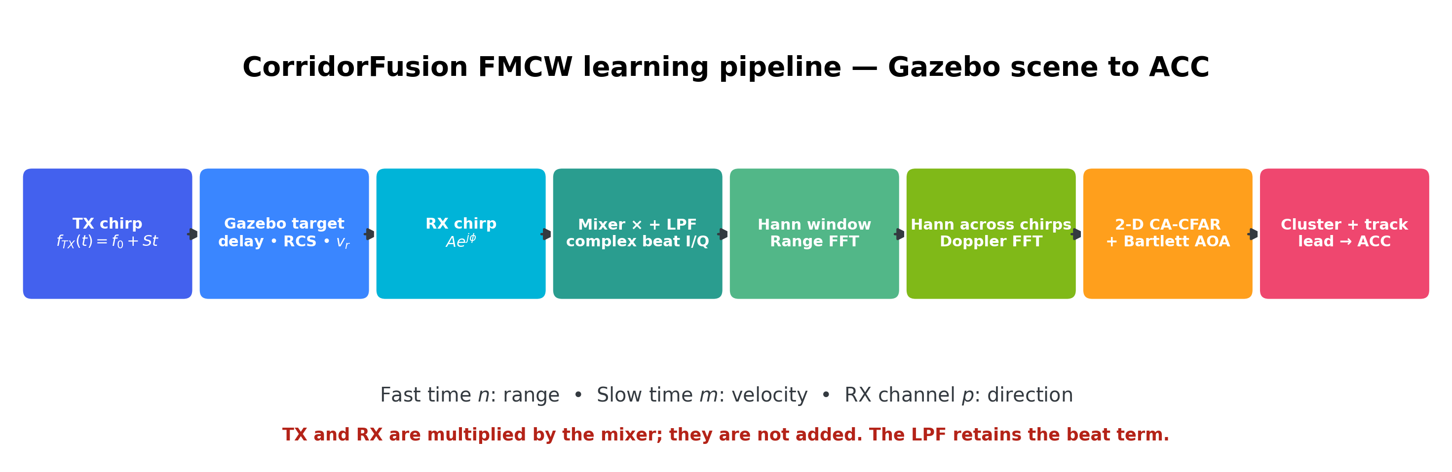
A complete detection
| Quantity | Comes from | Resolution |
|---|---|---|
| Range | Range FFT peak position | 0.600 m |
| Radial velocity | Doppler FFT peak bin | 0.760 m/s |
| Direction (AOA) | Phase across the RX array | 4 RX aperture |
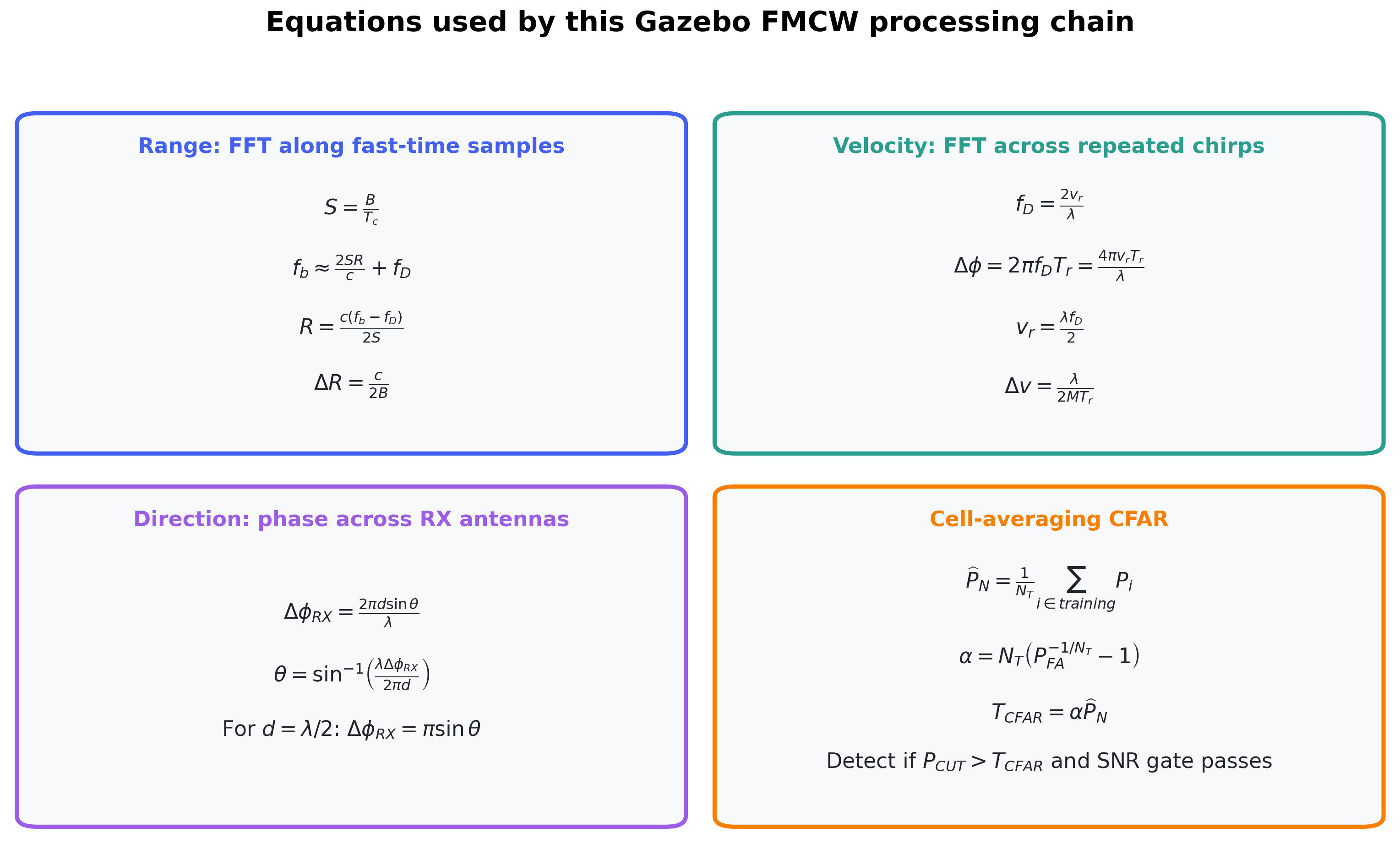
The main equations in one place
CFAR compares each candidate with its local background
Received power falls as the fourth power of range, so no single fixed threshold can serve both near and far targets. Cell-averaging CFAR estimates the noise locally and floats the threshold with it, which keeps the false-alarm rate constant across the whole map.
Cell under test
The candidate being judged.
Guard cells
Excluded from the noise estimate, because a real target spills energy into its neighbours and would otherwise raise its own bar.
Training cells
Averaged to estimate the local noise floor, then scaled by a factor derived from the desired false-alarm probability.
Cluster + gate
Surviving detections are merged in range, azimuth and Doppler so one vehicle produces one point rather than several.
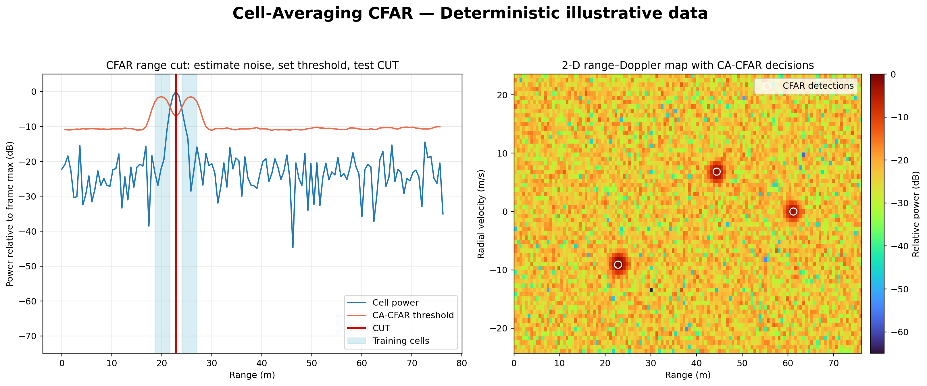
A cell scoring 50 with neighbours near 10 is a detection. The same score of 50 with neighbours near 46 is noise. Absolute magnitude carries no information on its own — only the contrast with its surroundings does.
From detections to an acceleration command
Detections become persistent objects in an EKF tracker, one filter per target with state x, y, vx, vy. The radial-velocity update is applied only along the line-of-sight direction, because radar cannot observe tangential motion and correcting both components would inject fictitious lateral velocity.
Lead selection then projects each confirmed track onto the ego vehicle's predicted path — an arc, not a straight line — and keeps the nearest one inside the lane corridor. On a curve this matters: a straight-line corridor test starts misclassifying adjacent-lane vehicles from roughly 30 m outward.
The following law
Desired gap is a constant time headway, 4.0 m + 1.8 s × v. Gaps that grow with speed are what make a platoon string stable. The acceleration request combines three terms: gap error, relative speed, and lead acceleration as feed-forward.
The relative-speed gain is several times the gap gain, so the largest gain in the loop multiplies the noisiest available signal. One Doppler bin flip becomes a step in the acceleration request — which is why velocity resolution, not range resolution, turned out to be the parameter that limited ride quality.